Erdős–Rényi Random Graph

• Notation: $G(n,p)$ or $\mathrm{ER}(n,p)$
• Model: Fixed $n$, undirected, $1\{(i,j)\in E\}\sim \mathrm{Bernoulli}(p)$
• Basic properties
  • $D_i\sim \mathrm{Binom}(n-1,p)\approx \mathrm{Poisson}(np)$
    • Also known as Poisson random graph model
  • $|E|\sim \mathrm{Binom}\left(\left(\genfrac{}{}{0ex}{}{n}{2}\right),p\right)$
  • Local Clustering: $\mathbb{E}{C}_i=p$
• Phase transitions
  • Edge existence: $t(n)=\frac{1}{n^2}$
  • Connectivity: $t(n)=\frac{\log n}{n}$
  • Giant component: $t(n)=\frac{1}{n}$
• Diameter: $\Theta (\ln n/\ln \lambda )$
  • see Diameter
• Sparse ER: $p_n=\lambda /n$
  • $D_i\approx \mathrm{Poisson}(\lambda )$
  • Number of $k$-cycles: $\Theta (1)$
  • Number of $k$-trees: $\Theta (n)$

Special Components

Analyzing the ER model requires us to calculate the probability of the existence of components of various shapes, or the expected number of them if they exist.

Singleton. Let $I_i^{(1)}$ be the indicator r.v. that $i$ is isolated and $I^{(1)}={\sum }_i{I}_i^{(1)}$. We have $\mathbb{E}[I^{(1)}]=n(1-p{)}^{n-1}$. The variance is calculated in the next section.

$k$-cycle. Randomly choose $k$ nodes, fix a starting node, and randomly arrange the rest $k-1$; they form a cycle if and only if they are only connected to the nodes before and after them. Thus, the expected number of $k$-cycles is

$$\mathbb{E}[I^{(k,\text{cycle})}]=\left(\genfrac{}{}{0ex}{}{n}{k}\right)\cdot (k-1)!\cdot \frac{1}{2}\cdot p^k\cdot (1-p{)}^{k(n-k)}\cdot (1-p{)}^{k(k-3)/2}.$$

Note that we have two $1/2$ factors: the first one is because a clockwise and a counter-clockwise arrangement of the same nodes correspond to the same cycle, and the second one is because the links between the $k$ nodes are double-counted by both ends. See Problem 5 for the calculation of the variance of $I^{(3,\text{cycle})}$.

$k$-tree. Randomly choose $k$ nodes and label them. Each possible tree formed by them has a unique Prüfer sequence¹ of length $k-2$. Thus, the number of possible trees is given by the Cayley’s formula $k^{k-2}$, and the expected number of $k$-trees is

$$\mathbb{E}[I^{(k,\text{tree})}]=\left(\genfrac{}{}{0ex}{}{n}{k}\right)\cdot k^{k-2}\cdot p^{k-1}\cdot (1-p{)}^{k(n-k)}\cdot (1-p{)}^{\left(\genfrac{}{}{0ex}{}{k}{2}\right)-(k-1)}.\text{\hspace{1em}(1)}$$

Connectivity

Let $p_n=\lambda \ln n/n$. We show that the network is connected w.p.1 if $\lambda >1$ and is disconnected w.p.1 if $\lambda <1$, as $n\to \infty$.

When $\lambda <1$, we inspect the probability of the existence of an isolated node. Then $\mathbb{E}[I^{(1)}]\to n^{1-\lambda }\to \infty$. The second moment of $I^{(1)}$ is

$$\mathbb{E}[(I^{(1)}{)}^2]=\mathbb{E}[I^{(1)}]+(n^2-n)\mathbb{E}[I_i^{(1)}{I}_j^{(1)}]\to n^{1-\lambda }+(n^2-n)n^{-2\lambda }.$$

Thus $\mathrm{Var}(I^{(1)})\to n^{1-\lambda }$. By the second Moment Method, we have $P(I^{(1)}\ge 1)\to 1$, and thus the network is disconnected w.p.1.

When $\lambda >1$, showing $P(I^{(1)}\ge 1)\to 0$ is not enough. We have to show that for any $k\ge 1$, the probability of the existence of a connected component of size $k$ goes to zero. Note that $k$ nodes form a standalone connected component only if they contain a spanning tree. Thus, similar to $(1)$, we have

$$\mathbb{E}[I^{(k)}]\le \left(\genfrac{}{}{0ex}{}{n}{k}\right)k^{k-2}{p}^{k-1}(1-p{)}^{k(n-k)}\lesssim n^{1-\lambda k}{k}^{k-2}{\lambda }^{k-1}\to 0,\forall k\ge 1.$$

By the union bound and Markov Inequality (or first Moment Method), we have

$$\begin{array}{rl}P(\text{disconnected})\le & \sum _{k=1}^{n/2}P(I^{(k)}\ge 1)\\ \le & \sum _{k=1}^{n/2}\mathbb{E}[I^{(k)}]\\ \le & \sum _{k=1}^{n/2}{n}^{1-\lambda k}{n}^{k-2}{\lambda }^{k-1}\\ =& n^{-1}\sum _{k=1}^{n/2}{n}^{-(\lambda -1)k}{\lambda }^{k-1}\\ \le & n^{-1}{n}^{-(\lambda -1)}\frac{1}{1-n^{-(\lambda -1)}\lambda }\\ \to & 0.\end{array}$$

A finer result captures the regime $p_n=\frac{\ln n+\alpha }{n}$:

$$P(\text{connected})\to e^{-e^{-\alpha }}.$$

Sparse ER

We call the ER model in the regime of $p_n=\lambda /n$ the sparse ER model (^dense-sparse). Note that the degree distribution approximates a Poisson Distribution with mean $\lambda$. Thus, this regime is also known as the Poisson random graph model.

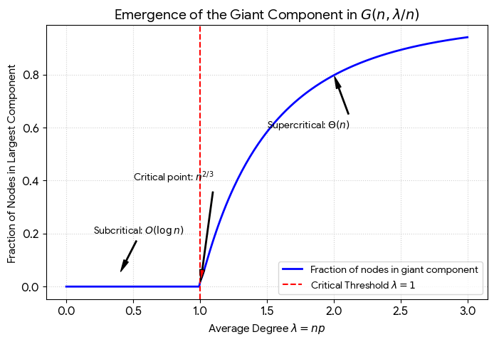
Subcritical regime $\lambda <1$. Let $C(i)$ be the connected component containing $i$. Then,

$$\mathbb{E}|C(i)|\to \frac{1}{1-\lambda }\text{and}P(\underset{i}{\max }|C(i)|=\Theta (\ln n))\to 1.$$

That is, the typical size of a component is $\frac{1}{1-\lambda }$, and the size of the largest component is $\Theta (\ln n)$.

Supercritical regime $\lambda >1$. Let $C_1$ be the largest component and $C_2$ be the second largest component. Let $\eta (\lambda )$ be the extinction probability of a Branching process with offspring distribution $\mathrm{Poisson}(\lambda )$. Then,

$$P(|C_1|=\Theta ((1-\eta (\lambda ))n))\to 1,P(|C_2|=O(\ln n))\to 1,\text{and}\mathbb{E}|C(i)|\to \frac{1}{1-\eta (\lambda )\lambda }.$$

That is, a giant component emerges with size $\Theta (n)$, the size of the second largest component is $\Theta (\ln n)$, and the typical size of a small component is $\frac{1}{1-\eta (\lambda )\lambda }$.

Proofs

Supercritical regime, giant component

Let $u$ be the probability that a random node $i$ does not belong to the giant component. Then $(1-u)n$ is the expected size of the giant component. We have the recursion

$$u=(1-p+pu{)}^{n-1},$$

where for any other node $j$, w.p. $1-p$, $i$ is not connected to $j$, and if they are connected, w.p. approximately $u$, $j$ does not belong to the giant component. Plugging $p=\lambda /n$ gives

$$u={\left(1+\frac{\lambda (u-1)}{n}\right)}^{n-1}\to \exp (\lambda (u-1))=g(u),$$

where $g$ is the PGF of $\mathrm{Poisson}(\lambda )$.

Regimes

Supercritical regime, uniqueness of the giant component

Before proving the second largest component in the supercritical regime is small, we can easily show that there cannot be two giant components. For any $v_1,v_2\in (0,1]$, suppose there are two giant components of sizes at least $v_{1}n$ and $v_{2}n$. The probability that they are not connected is at most $(1-p{)}^{v_{1}n\cdot v_{2}n}\to \exp (-\lambda v_1{v}_{2}n)$. Then, one can calculate the upper bound of the probability that there are two giant components using a similar equation in $(1)$.

Another easier approach is called sprinkling. Consider the ER model is generated in two steps: first generate links i.i.d. with probability $p$, and then sprinkle additional links with probability $n^{-ϵ}p$ for some small $ϵ\in (0,1)$. Then, this model is equivalent to $G(n,(1+n^{-ϵ})p)\to G(n,p)$.

Now suppose in the first step there are two giant components with sizes at least $v_{1}n$ and $v_{2}n$. Then, the probability that they are not connected in the second step is at most $(1-n^{-ϵ}p{)}^{v_{1}n\cdot v_{2}n}\to \exp (-\lambda v_1{v}_2{n}^{1-ϵ})\to 0$. Thus, w.p.1, $G(n,p)$ has only one giant component.

Supercritical regime, the second largest component

All regimes, typical size of a small component

We have proved in all regimes, there is at most one giant component with size $\Theta ((1-\eta (\lambda ))n)$, with $\eta (\lambda )=1$ when $\lambda <1$. For a random node $i$ not in the giant component, let $C(i)$ be the small component containing $i$. We have also proved that $|C(i)|=O(\ln n)$ almost surely and $C(i)$ is a tree almost surely. Thus, removing $i$ breaks $C(i)$ into $D_i$ subtrees, denoted by $\{C^{\prime }(j_k){\}}_{k=1}^{D_i}$. We have

$$|C(i)|=1+\sum _{k=1}^{D_i}|C^{\prime }(j_k)|,$$

which gives

$$\mathbb{E}|C(i)|=1+\mathbb{E}[D_i\mathbb{E}[C^{\prime }(j_1)\mid D_i]],$$

where we use the symmetry of the subtrees. In analogy to the Branching process, we have $\mathbb{E}[C^{\prime }(j_1)\mid D_i]=\mathbb{E}|C(i)|$. Additionally, note that $D_i$ links can only connect to nodes not in the giant component. Thus, $\mathbb{E}{D}_i=\eta np$. Together, we have

$$\mathbb{E}|C(i)|\to \frac{1}{1-\eta (\lambda )\lambda }.$$

See Local Branching for a more formal treatment.

Average size of small components

The above quantity is the expected size of a small component to which a random node belongs. It is not equivalent to the expected size of a randomly chosen small component. Since nodes in larger small components are more likely to be chosen, the above is larger than the average size of a randomly chosen small component.

Footnotes

1. Starts with an empty sequence, remove the leaf node with the smallest label and append the label to the sequence, and repeat until only two nodes are left. The Prüfer sequence of a $k$-tree has a length $k-2$ and is a bijection. ↩