Matlab Graphics - Scatter Plots

Scatter Plots

MATLAB Graphics

---

散点图 scatter plots 是 MATLAB 中一基本图形, class 为 matlab.graphics.chart.primitive.Scatter

Functions

• 2-D: scatter
• 3-D: scatter3, 用法同 scatter

Scatter Properties

散点图性质 scatter properties 控制 Scatter object 的样貌和表现, 以 structure 类储存. 通过将图像以对象 object 形式储存在变量中, 可以查看和修改其各种性质

p =
 
  Scatter with properties:
 
             Marker: 'o'
    MarkerEdgeColor: 'none'
    MarkerFaceColor: 'flat'
           SizeData: [1x200 double]
          LineWidth: 0.5000
              XData: [1x200 double]
              YData: [1x200 double]
              ZData: [1x0 double]
              CData: [1x200 double]
 
  Use GET to show all properties

以下列出部分 Marker 性质.

Marker Symbol

• Field name: .Marker
• Default: 'o'
• Inputs: same as Marker Symbol

Width of marker edge

• Field name: .LineWidth
• Default: 0.5
• Inputs: numeric

Marker Outline Color

• Field name: .MarkerEdgeColor
• Default: 'flat'
• Inputs: 'flat', an RGB triplet, a hexadecimal color code, a color name, or a short name
  • The 'flat' option uses the CData values
  • The ‘auto’ option uses the same color as the Color property for the axes

Marker Fill Color

• Field name: .MarkerFaceColor
• Default: 'none'
• Inputs: 'flat', 'auto', an RGB triplet, a hexadecimal color code, a color name, or a short name
  • The 'flat' option uses the CData values
  • The 'auto' option uses the same color as the Color property for the axes

Marker Edge Transparency

• Field name: .MarkerEdgeAlpha
• Default: 1
• Inputs: scalar in range [0,1], 'flat'
  • To set the edge transparency to a different value for each point in the plot, set the AlphaData property to a vector the same size as the XData property, and set the MarkerEdgeAlpha property to 'flat'

Marker Face Transparency

• Field name: .MarkerFaceAlpha
• Default: 1
• Inputs: scalar in range [0,1], 'flat'

Examples

2-D

x = linspace(0,3*pi,200);
y = cos(x) + rand(1,200);
sz = linspace(1,25,length(x));
c = linspace(1,1000,length(x));
scatter(x,y,sz,c,'filled')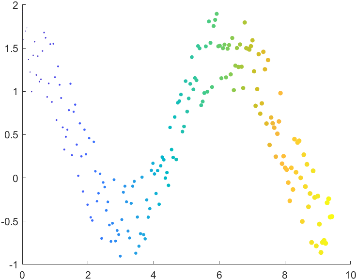

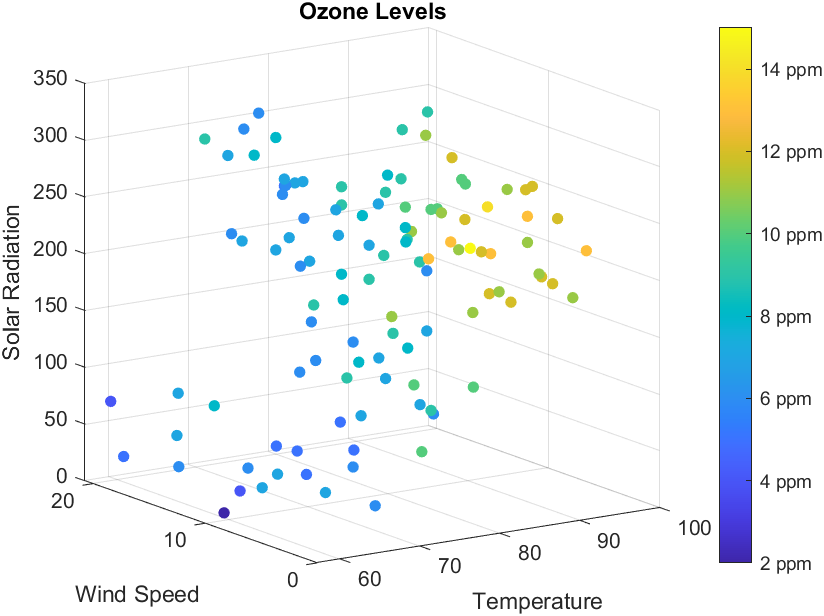
20210218121222

3-D

% Load data on ozone levels
load ozoneData Ozone Temperature WindSpeed SolarRadiation
% Calculate the ozone levels
z = (Ozone).^(1/3);
response = z;
% Make a color index for the ozone levels
nc = 16;
offset = 1;
c = response - min(response);
c = round((nc-1-2*offset)*c/max(c)+1+offset);
% Create a 3D scatter plot using the scatter3 function
figure
scatter3(Temperature, WindSpeed, SolarRadiation, 30, c, 'filled')
view(-34, 14)
% Add title and axis labels
title('Ozone Levels')
xlabel('Temperature')
ylabel('Wind Speed')
zlabel('Solar Radiation')
% Add a colorbar with tick labels
colorbar('Location', 'EastOutside', 'YTickLabel',...
    {'2 ppm', '4 ppm', '6 ppm', '8 ppm', ...
    '10 ppm', '12 ppm', '14 ppm'})

20210218122004