Ridge Regression

Ridge regression controls the modulus of the weight: we use Mean Squared Error plus L2 Regularization as the Cost Function

$$J=\Vert y-Xw{\Vert }^2+\alpha \Vert w{\Vert }^2=(Xw-y{)}^T(Xw-y)+\alpha w^{T}w$$

We get $w_{\text{symrm}RR}\to w_{\text{symrm}LS}$ as $\alpha \to 0$; and $w_{\text{symrm}RR}\to 0$ as $\alpha \to \infty$.

Then with the same process, we get

$$w=(X^{T}X+\alpha I{)}^{-1}{X}^{T}y.$$

image.png

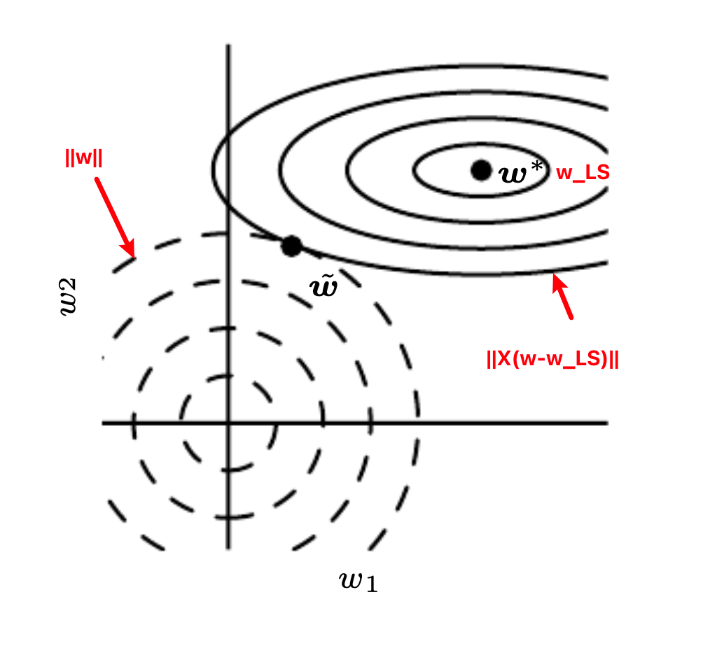
Above is an illustration. Ridge regression seeks an equilibrium between the weight norm and the MSE.

The math relationship between $w_{\text{symrm}RR}$ and $w_{\text{symrm}MLE}$ is derived in Weight Decay, where $\tilde{w}=w_{\text{symrm}RR}$ and $w^{\ast }=w_{\text{symrm}LS}$; $H=X^{T}X=Q\Lambda Q^T$ is the eigenvalue decomposition/SVD. Furthermore, let $X=US{V}^T$, we have

$$\{\begin{array}{ll}{w}_{\text{symrm}RR}& =V\text{diag}\left\{\frac{{\sigma }_i}{\alpha +{\sigma }_i^2}\right\}{U}^{T}y;\\ w_{\text{symrm}LS}& =V\text{diag}\{{\sigma }_i^{-1}\}{U}^{T}y.\end{array}$$

Therefore, ridge regression is more stable than Linear Regression.

Also, we can see that L2 Regularization causes the learning algorithm to “perceive” the input $X$ as having a higher variance, which makes it shrink the weights on features whose covariance with the output target is low compared to this added variance.

In the above example, the components of $X$ corresponding to the first dimension $w_1$ has lower variance (or the eigenvalue of the Hessian of $J$ is small in this direction); thus, the objective function does not increase much when moving horizontally away from $w_{\text{symrm}LS}$. Then the regularizer pulls $w_1$ close to zero. In the second dimension, the situation is reversed, pulling $w_2$ away from zero.

Pseudoinverse

As we can see, if we let $\alpha \to 0$, then we get

$w=X^{†}y$

where $X^{†}$ is the Moore-Penrose Pseudoinverse. Therefore we can interpret the pseudoinverse as stabilizing underdetermined problems using regularization.

Variance, Correlation, Singular Value, and Weight

First, the variance of the random vector is a Covariance matrix. And the sample Covariance matrix is $\frac{1}{n-1}{X}^{T}X$. For highly correlated data, i.e., some features are dependent, some non-diagonal elements of the covariance matrix will be big. Also, if the data is correlated, some eigenvalues of $X^{T}X$ or singular values of $X$ will be small.

Back to the illustrative graph above. We know that

$$J_{\text{symrm}LS}(w)=\Vert y-Xw{\Vert }^2=\Vert y-X{w}_{\text{symrm}LS}{\Vert }^2+\Vert X(w-w_{\text{symrm}LS}){\Vert }^2,$$

and

$${\nabla }_w{J}_{\text{symrm}LS}(w)=2X^{T}X(w-w_{\text{symrm}LS}),$$

which is zero at $w_{\text{symrm}LS}$. Therefore, we need to examine the Hessian of $J$, which is $2X^{T}X$, the scaled sample Covariance matrix.

So the sample Covariance matrix determines the curvature of $J_{\text{symrm}LS}$ at $w_{\text{symrm}LS}$. And $J_{\text{symrm}LS}$ is more sensitive in directions of $w$ corresponding to larger eigenvalues of $X^{T}X$, or larger singular values of $X$, which captures larger variance of the data.

Then, with regularization, $w$‘s direction with a smaller variance will be pull to zero more quickly.

Bias and Variance

$$\mathbb{E}[w_{\text{symrm}RR}]=(\lambda I+X^{T}X{)}^{-1}{X}^{T}Xw,\mathrm{Var}(w_{\text{symrm}RR})={\sigma }^{2}Z(X^{T}X{)}^{-1}{Z}^T,$$

where $Z=(I+\lambda (X^{T}X{)}^{-1}{)}^{-1}$.

Compared to the variance of $w_{\text{symrm}MLE}$:

\begin{aligned}
\Var\[w\_{\mathrm{MLE}}]
\=& \mathbb{E}\[w\_{\mathrm{MLE}}w\_{\mathrm{MLE}}^{T}] - \mathbb{E}\[w\_{\mathrm{MLE}}]\mathbb{E}\[w\_{\mathrm{MLE}}]^{T}\\
\= & \mathbb{E}\left\[\left(X^T X\right)^{-1} X^T Y Y^T X\left(X^T X\right)^{-1}\right]-w w^T \\
\= & \left(X^T X\right)^{-1} X^T \mathbb{E}\left\[Y Y^T\right] X\left(X^T X\right)^{-1}-w w^T \\
\= & \left(X^T X\right)^{-1} X^T (\Var(Y) + \mathbb{E}\[Y]\mathbb{E}\[Y]^{T}) X\left(X^T X\right)^{-1}-w w^T \\
\= & \left(X^T X\right)^{-1} X^T\left(\sigma^2 I+X w w^T X^T\right) X\left(X^T X\right)^{-1}-w w^T \\
\= & \left(X^T X\right)^{-1} X^T \sigma^2 I X\left(X^T X\right)^{-1}+ \\
& \left(X^T X\right)^{-1} X^T X w w^T X^T X\left(X^T X\right)^{-1}-w w^T \\
\= & \sigma^2\left(X^T X\right)^{-1}\\
\= & \sigma^{2}V\Sigma ^{-2}V^{T},
\end{aligned}

Link to original

the variance of $w_{\text{symrm}MLE}$ shrinks by a factor of $(1+\lambda C{)}^{-1}$.

Least Squares vs. Ridge Regression

• Least squares solution: unbiased, but potentially high variance
• Ridge regression solution: biased, but lower variance than LS

For general bias and variance trade-off, see Bias-Variance Trade-Off.