Expectation Maximization

Expectation Maximization (EM) algorithm is an iterative algorithm used to estimate the Maximum Likelihood Estimation (MLE) or Maximum a Posteriori (MAP) parameters of a probabilistic model, in the presence of unobserved or missing data.

Imagine we have a hidden (unobserved or missing) random variable $Y$, given whose observation the Likelihood $p(x,y\mid \theta )$ is easy to compute or optimize. When only $x$ is available, we take the expectation over $Y$:

$$p(x\mid \theta )={\int }_{\mathcal{Y}}p(x,y\mid \theta )\mathrm{d}y.$$

Then, optimizing the RHS gives us the MLE/MAP.

Missing Gaussian Data

For a Gaussian random variable $X$ with observed subvector $x^o$ and missing subvector $x^m$, we can easily find its Maximum Likelihood Estimation for parameters when there is no missing data. Therefore, with the presence of missing data, we have

$$p\left(x_i^o\mid \mu ,\Sigma \right)=\int p\left(x_i^o,x_i^m\mid \mu ,\Sigma \right)d{x}_i^m=N\left({\mu }_i^o,{\Sigma }_i^o\right),$$

where ${\mu }_i^o$ and ${\Sigma }_i^o$ are the sub-vector/sub-matrix of $\mu$ and $\Sigma$ defined by $x_i^o$.

Mixture of Gaussians

For the mixture of two Gaussian distributions $\mathcal{N}({\mu }_1,1)$ and $\mathcal{N}({\mu }_2,1)$, it can be think of that the random variable first pick a Gaussian distribution with probability $0.5$, and then sample from the selected Gaussian. Under this interpretation, the hidden variable $Y\sim \mathrm{Bernoulli}(0.5)$ is the index of the selected Gaussian. Then, $X=Y{Z}_1+(1-Y)Z_2$, where $Z_1\sim \mathcal{N}({\mu }_1,1)$ and $Z_2\sim \mathcal{N}({\mu }_2,1)$.

With the help of this auxiliary variable $Y$, the log-likelihood function changed from

$$\ln p(x\mid {\mu }_1,{\mu }_2)=\ln \left(\exp (-(x-{\mu }_1{)}^2/2)+\exp (-(x-{\mu }_2{)}^2)/2\right),$$

which is neither convex nor concave in ${\mu }_1$ and ${\mu }_2$, to

$$\begin{array}{rl}\ln p(x,y\mid {\mu }_1,{\mu }_2)+const.=& \ln \left(y\exp (-(x-{\mu }_1{)}^2/2)+(1-y)\exp (-(x-{\mu }_2{)}^2)/2\right)\\ =& \ln \left(\exp (-y(x-{\mu }_1{)}^2/2-(1-y)(x-{\mu }_2{)}^2)/2\right)\\ =& -\frac{1}{2}(y(x-{\mu }_1{)}^2+(1-y)(x-{\mu }_2{)}^2),\end{array}$$

which is concave in ${\mu }_1$ and ${\mu }_2$.

More often, the Log-Likelihood function, which is a summation instead of a production, is easier to optimize given complete data: $\log p(x,y\mid \theta )$. This motivates the EM algorithm.

Objective Justification

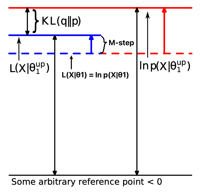
Decomposition

Formally, with the help of another random variable $y$ and its distribution $q$, we have the following log-likelihood decomposition:

$$\begin{array}{rl}\ln p(x|\theta )=& {\int }_{\mathcal{Y}}q(y)\ln p(x|\theta )\mathrm{d}y\\ =& {\int }_{\mathcal{Y}}q(y)\ln \frac{p(x,y|\theta )}{p(y|x,\theta )}\mathrm{d}y\\ =& {\int }_{\mathcal{Y}}q(y)\ln p(x,y|\theta )\mathrm{d}y-{\int }_{\mathcal{Y}}q(y)\ln p(y|x,\theta )\mathrm{d}y\\ =& {\mathbb{E}}_q[\ln p(x,Y\mid \theta )]+H(q\Vert p_{x,\theta }),\end{array}$$

where $p_{x,\theta }$ is the conditional distribution of $y$ given $x$ and $\theta$, and $H$ is the Cross-Entropy.

Should we maximize or minimize the entropy term in the above decomposition?

Since we want to maximize the log-likelihood, the above decomposition seems to suggest that we should maximize the cross-entropy over $q$. However, it’s important to note that the above equality holds for any $q$. And thus $q$ is not a decision variable.

Instead, we notice that

$$\begin{array}{rl}\ln p(x\mid \theta )=& {\mathbb{E}}_q[\ln p(x,Y\mid \theta )]+D_{\mathrm{KL}}(q\Vert p_{x,\theta })-{\mathbb{E}}_q[\ln q(Y)]\\ \ge & {\mathbb{E}}_q[\ln p(x,Y\mid \theta )]-\underset{\text{constant w.r.t. }\theta }{\underbrace{{\mathbb{E}}_q[\ln q(Y)]}},\end{array}$$

because the KL Divergence is always non-negative. Therefore, we see that when optimizing the log-likelihood over $\theta$, the increase of the objective will be lower bounded by the increase of the expectation term ${\mathbb{E}}_q[\ln p(x,Y\mid \theta )]$, which is easier to optimize as it involves the log-likelihood of the complete data $(X,Y)$. And to make this lower bound tight, we need to minimize the Cross-Entropy/KL Divergence term. By this, any increase in the expectation term leads to the maximum increase in the log-likelihood.

Another reason for minimizing the cross-entropy term is given in Convergence Property.

Lower Bound

We can also use the marginalization/expectation in ^eq-margin for log-likelihood. To do this, we need to introduce an arbitrary distribution $q$ for $y$ and uses Jensen’s inequality:

$$\begin{array}{rl}\ln p(x\mid \theta )=& \ln {\int }_{\mathcal{Y}}p(x,y\mid \theta )\mathrm{d}y\\ =& \ln {\int }_{\mathcal{Y}}\frac{p(x,y\mid \theta )}{q(y)}q(y)\mathrm{d}y\\ =& \ln {\mathbb{E}}_q\left[\frac{p(x,Y\mid \theta )}{q(y)}\right]\\ \ge & {\mathbb{E}}_q\left[\ln \frac{p(x,Y\mid \theta )}{q(y)}\right]\\ =& {\mathbb{E}}_q\left[\ln p(x,Y\mid \theta )\right]+H(q).\end{array}$$

Similarly, to make any increase in the expectation term lead to the maximum increase in the log-likelihood, we need the equality to hold, which requires

$$q(y)\propto p(x,y\mid \theta )⟹q(y)=\frac{p(x,y\mid \theta )}{\int p(x,y\mid \theta )\mathrm{d}y}=\frac{p(y\mid x,\theta )p(x\mid \theta )}{\int p(y\mid x,\theta )p(x\mid \theta )\mathrm{d}y}=p_{x,\theta }(y).$$

Algorithm

Justified above, the EM algorithm iteratively minimizes the cross-entropy term and then maximizes the expectation term:

1. E-step: Update

$$q_{t+1}=\underset{q}{\mathrm{argmin}}H(q\Vert p_{x,{\theta }_t})=p_{x,{\theta }_t},$$

and calculate the expectation ${\mathbb{E}}_{q_{t+1}}\ln p\left(x,Y\mid \theta \right)$. 2. M-step: Update

$${\theta }_{t+1}=\arg \underset{\theta }{\max }{\mathbb{E}}_{q_{t+1}}[\ln p\left(x,Y\mid \theta \right)].$$

Convergence Property

Generally, EM is not theoretically guaranteed to converge to the Maximum Likelihood Estimation or Maximum a Posteriori. However, it is a monotonic increasing algorithm:

$$\begin{array}{rlrl}\ln p(x\mid {\theta }_t)& ={\mathbb{E}}_q\ln p(x,Y\mid {\theta }_t)+H(q\Vert p_{x,{\theta }_t})& & \text{(holds for any q)}\\ & ={\mathbb{E}}_{q_{t+1}}\ln p(x,Y\mid {\theta }_t)+H(q_{t+1}\Vert p_{x,{\theta }_t})& & \\ & ={\mathbb{E}}_{q_{t+1}}\ln p(x,Y\mid {\theta }_t)+H(q_{t+1})& & \text{(E-step; H(q) is self-entropy)}\\ & \le {\mathbb{E}}_{q_{t+1}}\ln p(x,Y\mid {\theta }_{t+1})+H(q_{t+1})& & \text{(M-step)}\\ & \le {\mathbb{E}}_{q_{t+1}}\ln p(x,Y\mid {\theta }_{t+1})+H(q_{t+1}\Vert p_{x,{\theta }_{t+1}})& & (H(q\Vert p)>H(q)\text{ if }p\ne q)\\ & ={\mathbb{E}}_q\ln p(x,Y\mid {\theta }_{t+1})+H(q\Vert p_{x,{\theta }_{t+1}})& & \text{(holds for any q)}\\ & =\ln p(x\mid {\theta }_{t+1}).& & \end{array}$$

Note that we have two increases in one iteration: Additionally, the increase in the cross-entropy/KL term is introduced by the update of $\theta$ rather than $q$. And to make any update in $\theta$ lead to an increase in the cross-entropy/KL term, we need to first minimize the cross-entropy/KL term in the E-step. This reasoning is consistent with Objective Justification.

Application: Mixed Gaussian Model

Continuing the mixture of Gaussians example, we see that given the hidden observation $\{y_i{\}}_{i=1}^n$, we can easily calculate the log-likelihood maximizer:

$${\hat{\mu }}_1=\frac{{\sum }_i{x}_i{y}_i}{{\sum }_i{y}_i},{\hat{\mu }}_2=\frac{{\sum }_i{x}_i(1-y_i)}{{\sum }_i(1-y_i)}.$$

Without direct observation, we replace them with expectation:

$${\mathbb{E}}_Y\ln p(x,Y\mid \mu )=-n\ln (2\sqrt{2\pi })-\frac{1}{2}\sum _{i=1}^n\left[\mathbb{E}[Y_i](x_i-{\mu }_1{)}^2+(1-\mathbb{E}[Y_i])(x_i-{\mu }_2{)}^2\right].$$

Setting the distribution of $Y_i$ as $p_{x_i,\mu }$ gives the E-step:

$$\begin{array}{rl}\mathbb{E}{Y}_i=& P(Y_i=1\mid x_i,\mu )=\frac{P(Y_i=1,x_i\mid \mu )}{P(x_i\mid \mu )}\\ =& \frac{\exp (-(x_i-{\mu }_1{)}^2/2)\cdot 1/2}{\exp (-(x_i-{\mu }_1{)}^2/2)\cdot 1/2+\exp (-(x_i-{\mu }_2{)}^2/2)\cdot 1/2}\\ =& \frac{1}{1+\exp (((x_i-{\mu }_1{)}^2-(x_i-{\mu }_2{)}^2)/2)},\end{array}$$

which is larger than 0.5 if $x_i$ is closer to ${\mu }_1$, and smaller than 0.5 if $x_i$ is closer to ${\mu }_2$. Then, the M-step is to maximize the expectation:

$${\hat{\mu }}_1=\frac{{\sum }_{i=1}^n\mathbb{E}[Y_i]x_i}{{\sum }_{i=1}^n\mathbb{E}[Y_i]},{\hat{\mu }}_2=\frac{{\sum }_{i=1}^n(1-\mathbb{E}[Y_i])x_i}{{\sum }_{i=1}^n(1-\mathbb{E}[Y_i])}.$$

Application: Filling Missing Gaussian Data

We now return to the example of missing Gaussian data, to both learn the parameter and fill in the missing data. In this specific problem $\theta =(\mu ,\Sigma ),y=x^m$. And the objective decomposition reads

$$\begin{array}{rl}\sum _{i=1}^n\ln p\left(x_i^o\mid \mu ,\Sigma \right)=& \sum _{i=1}^n\int q\left(x_i^m\right)\ln \frac{p\left(x_i^o,x_i^m\mid \mu ,\Sigma \right)}{q\left(x_i^m\right)}d{x}_i^m+\\ & \sum _{i=1}^n\int q\left(x_i^m\right)\ln \frac{q\left(x_i^m\right)}{p\left(x_i^m\mid x_i^o,\mu ,\Sigma \right)}d{x}_i^m.\end{array}$$

As we can see, the only difficult part is calculating $q=p(x^m|x^o,\mu ,\Sigma )$.

For the E-step, since $[x_i^o;x_i^m]\sim \mathcal{N}(\mu ,\Sigma )$, by Normal Marginal Distribution from Normal Joint Distribution, we get the conditional parameter of ^q:

$${\hat{\mu }}_i={\mu }_i^m+{\Sigma }_i^{mo}{\left({\Sigma }_i^{oo}\right)}^{-1}\left(x_i^o-{\mu }_i^o\right),{\hat{\Sigma }}_i={\Sigma }_i^{mm}-{\Sigma }_i^{mo}{\left({\Sigma }_i^{oo}\right)}^{-1}{\Sigma }_i^{om}$$

For the M-step, we need to maximize the following expectation:

$$\begin{array}{rl}{\mathbb{E}}_q[\ln (p(x_i^o,x_i^m|\mu ,\Sigma ))]=& {\mathbb{E}}_q[(x_i-\mu {)}^T{\Sigma }^{-1}(x_i-\mu )]\\ =& {\mathbb{E}}_q[\mathrm{trace}\{{\Sigma }^{-1}(x_i-\mu )(x_i-\mu {)}^T\}]\\ =& \mathrm{trace}\{{\Sigma }^{-1}{\mathbb{E}}_q[(x_i-\mu )(x_i-\mu {)}^T]\}\end{array},$$

where $q(x_i^m)=\mathcal{N}({\hat{\mu }}_i,{\hat{\Sigma }}_i)$. Then the maximization gives us

$$\begin{array}{rl}{\mu }_{\mathrm{up}}& =\frac{1}{n}\sum _{i=1}^n{\hat{x}}_i,\\ {\Sigma }_{\mathrm{up}}& =\frac{1}{n}\sum _{i=1}^n\left(\left({\hat{x}}_i-{\mu }_{\mathrm{up}}\right){\left({\hat{x}}_i-{\mu }_{\mathrm{up}}\right)}^T+{\hat{V}}_i\right),\end{array}$$

where ${\hat{x}}_i$ is $x_i$ with the missing values being replaced by ${\hat{\mu }}_i$, and ${\hat{V}}_i$ is the zeros matrix plus the sub-matrix ${\hat{\Sigma }}_i$ in the missing dimensions.