M-Estimator

For an Estimation task, one can have different objectives (or metrics). For example, MLE maximizes the likelihood of the estimator, Least Squares minimizes its squared error, and Ridge Regression minimizes the squared error with a penalty term.

M-estimators generalize the above ideas by using a general objective function,

$$m:\Theta \times \mathcal{X}\to \overline{\mathbb{R}},(\theta ,x)\mapsto m_{\theta }(x).$$

Then, we can define the empirical error: $M_n(\theta ):={\hat{\mathbb{E}}}_n{m}_{\theta }(X)=\frac{1}{n}{\sum }_{i=1}^n{m}_{\theta }(x_i)$, a.k.a. the criterion function. And an M-Estimator minimizes the empirical error:

$$\hat{\theta }=\underset{\theta \in \Theta }{\mathrm{argmin}}{M}_n(\theta ).$$

• 💡 We can see that M-estimators and Empirical Risk Minimization have the same formulation, one in the context of Estimation and the other in the context of Prediction/Supervised Learning.

Examples

We only need to specify the $m$ function to get different M-estimators.

• Maximum Likelihood Estimation: $m_{\theta }(x)=-\log p_{\theta }(x)$.
• Ordinary Least Squares: $m_{\theta }(x)=(y-x^T\theta {)}^2$.
• Ridge Regression: $m_{\theta }(x)=(y-x^T\theta {)}^2+\lambda \Vert \theta {\Vert }^2$.
• Median regression: $m_{\theta }(x)=|y-x^T\theta |$.
• Quantile regression: $m_{\theta }(x)=-(\theta -x)(\tau -1(\theta -x>0))$.
  • This loss is also known as the pinball loss.

Properties

In this section, we denote $M(\theta ):={\mathbb{E}}_P{m}_{\theta }(X)$, and

$${\theta }^{\ast }=\underset{\theta \in \Theta }{\mathrm{argmin}}M(\theta ).$$

Consistency

By LLN, we know that

$$M_n(\theta )\stackrel{P/\text{a.s.}}{\to }M(\theta ),\forall \theta .$$

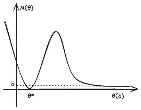
We wonder under what conditions the following is also true

$$\hat{\theta }:=\underset{\theta \in \Theta }{\mathrm{argmin}}{M}_n(\theta )\stackrel{P}{\to }\underset{\theta \in \Theta }{\mathrm{argmin}}M(\theta )=:{\theta }^{\ast }.$$

In the function graph of $M$ and $M_n$ (see e.g. ^fig-m-graph), the question ask what conditions allow to transfer the convergence of y-axis to that of x-axis.

It turns out that the above consistency holds under two reasonable conditions:

• Uniform convergence: ${\sup }_{\theta \in \Theta }|M_n(\theta )-M(\theta )|\stackrel{P}{\to }0$.

  • Some sufficient conditions for uniform convergence:
    • Finite VC dimension.
    • Finite Rademacher Complexity or Gaussian Complexity.
    • Compact $\Theta$ and continuous $M_{\theta }$ and $M$, and ${\mathbb{E}}_P[{\sup }_{\theta \in \Theta }{M}_{\theta }(X)]<\infty$.

• Separation: For any $ϵ$, ${\inf }_{\theta :\Vert \theta -{\theta }^{\ast }\Vert >ϵ}M(\theta )>M({\theta }^{\ast })$

  • 💡 In words, this condition says that only parameters close to ${\theta }^{\ast }$ may yield a value of $M(\theta )$ close to the minimum $M({\theta }^{\ast })$.

Example of M function whose point of maximum is not well separated.

Proof of Consistency

By the definition of $\hat{\theta }$, we have the critical inequality:

$$M_n(\hat{\theta })\le M_n({\theta }^{\ast })\stackrel{P}{\to }M({\theta }^{\ast }).$$

Thus, we have

$$M_n(\hat{\theta })\le M({\theta }^{\ast })+o_P(1).\text{\hspace{1em}(1)}$$

By the uniform convergence condition,

$$\begin{array}{rl}M(\hat{\theta })-M({\theta }^{\ast })\le & M(\hat{\theta })-(M_n(\hat{\theta })-o_P(1))\\ \le & \underset{\hat{\theta }\in \Theta }{\sup }|M(\hat{\theta })-M_n(\hat{\theta })|+o_P(1)\\ \stackrel{P}{\to }& 0.\end{array}$$

Then, since no other parameter can yield a value of $M(\theta )$ close to $M({\theta }^{\ast })$ by the separation condition, we know $\hat{\theta }\stackrel{P}{\to }{\theta }^{\ast }$. More specifically, for any $ϵ>0$, we have

$$\delta :=\underset{\theta :\Vert \theta -{\theta }^{\ast }\Vert >ϵ}{\inf }M(\theta )-M({\theta }^{\ast })>0.$$

Then, since $M(\hat{\theta })-M({\theta }^{\ast })\stackrel{P}{\to }0$, we know that $\Vert \hat{\theta }-{\theta }^{\ast }\Vert \stackrel{P}{\le }ϵ$. By the arbitrariness of $ϵ$, we get the result.

Consistency of Approximate Estimator

As we can see in the proof, the crucial step is $(1)$. Therefore, we can replace $\hat{\theta }$ by any approximate estimator $\tilde{\theta }$ (approximate minimizer of $M_n$), and its consistent as long as $(1)$ holds, or equivalently,

$$\begin{array}{rl}& M_n(\tilde{\theta })\le M_n(\hat{\theta })+o_P(1)\\ ⟹& M_n(\tilde{\theta })\le M({\theta }^{\ast })+o_P(1).\end{array}$$

Asymptotic Normality

Under some regularity conditions:

• $\theta \mapsto m_{\theta }(x)$ is differentiable at ${\theta }^{\ast }$ $P$-a.s. (for almost every $x$);
• There exists an $L_2$ function $f$, such that $|m_{{\theta }_1}(x)-m_{{\theta }_2}(x)|\le f(x)\Vert {\theta }_1-{\theta }_2\Vert$ for all ${\theta }_1,{\theta }_2$ in a neighborhood of ${\theta }^{\ast }$;
• $e:\theta \mapsto \mathbb{E}{m}_{\theta }(X)$ is twice differentiable with a non-singular second derivative at ${\theta }^{\ast }$, denoted as $V_{{\theta }^{\ast }}={\ddot{e}}_{{\theta }^{\ast }}$;

we have

$$\sqrt{n}\left(\hat{\theta }-{\theta }^{\ast }\right)\stackrel{d}{\to }\mathcal{N}(0,V_{{\theta }^{\ast }}^{-1}\mathbb{E}[{\dot{m}}_{{\theta }^{\ast }}{\dot{m}}_{{\theta }^{\ast }}^T]V_{{\theta }^{\ast }}^{-1}).$$

• ❗️ Note that we do not require $m_{\theta }$ is twice differentiable. The twice differentiability of $e$ is weaker.

Proof Sketch

In the proof sketch, we neglect the expectation, and assume that the expectation and derivatives commute. By Taylor expansion,

$$M(\theta )-M({\theta }^{\ast })\approx {\dot{M}}_{{\theta }^{\ast }}^T(\theta -{\theta }^{\ast })+\frac{1}{2}(\theta -{\theta }^{\ast }{)}^T{\ddot{M}}_{{\theta }^{\ast }}(\theta -{\theta }^{\ast }).$$

Denote the RHS as $Q(\theta )$. Then, we have

$$\hat{\theta }\approx \underset{\theta }{\mathrm{argmin}}M(\theta )\approx \underset{\theta }{\mathrm{argmin}}Q(\theta ).$$

By setting

$$\dot{Q}(\theta )={\dot{M}}_{{\theta }^{\ast }}+{\ddot{M}}_{{\theta }^{\ast }}(\theta -{\theta }^{\ast })=0,$$

we get

$$\hat{\theta }-{\theta }^{\ast }\approx -{\ddot{M}}_{{\theta }^{\ast }}^{-1}{\dot{M}}_{{\theta }^{\ast }}.$$

Thus, the asymptotic variance is approximately

$${\ddot{M}}_{{\theta }^{\ast }}^{-1}{\dot{M}}_{{\theta }^{\ast }}{\dot{M}}_{{\theta }^{\ast }}^T{\ddot{M}}_{{\theta }^{\ast }}^{-1}=V_{{\theta }^{\ast }}^{-1}\mathbb{E}[{\dot{m}}_{{\theta }^{\ast }}{\dot{m}}_{{\theta }^{\ast }}^T]V_{{\theta }^{\ast }}^{-1}.$$

Asymptotic Normality of Quantile Regression

Treating quantile regression as an M-estimator, we verify the above conditions and establish its asymptotic normality. Recall the pinball loss function:

$$m_{\theta }(x)=-(\theta -x)(q-1\{\theta -x>0\}).$$

For the first condition, $\frac{\partial }{\partial \theta }{m}_{\theta }(x){|}_{{\theta }^{\ast }}$ exists if $x\ne {\theta }^{\ast }$. For any continuous distribution, $P(X={\theta }^{\ast })=0$, so the first condition holds, and ${\dot{m}}_{\theta }(x)=-q+1\{\theta >x\}$.

The second condition also holds:

$$\begin{array}{rl}|m_{{\theta }_1}(x)-m_{{\theta }_2}(x)|& =\left|q({\theta }_2-{\theta }_1)+({\theta }_1-x)1\{{\theta }_1>x\}-({\theta }_2-x)1\{{\theta }_2>x\}\right|\\ & \le q\left|{\theta }_2-{\theta }_1|+|({\theta }_1-x)1\{{\theta }_1>x\}-({\theta }_2-x)1\{{\theta }_2>x\}\right|\\ & \le q|{\theta }_1-{\theta }_2|+|{\theta }_1-{\theta }_2|\\ & =(q+1)|{\theta }_1-{\theta }_2|.\end{array}$$

For the third condition, we have

$$\begin{array}{rl}e(\theta )=& {\int }_{-\infty }^{\theta }(1-q)(\theta -x)p(x)\mathrm{d}x-{\int }_{\theta }^{\infty }q(\theta -x)p(x)\mathrm{d}x\\ =& -q\theta +q\mathbb{E}[X]+\theta F(\theta )-{\int }_{-\infty }^{\theta }xp(x)\mathrm{d}x\end{array}$$

By integration by parts,

$$e(\theta )=q(\theta -\mu )+\theta F(\theta )-\left(xF(x){|}_{-\infty }^{\theta }-{\int }_{-\infty }^{\theta }F(x)\mathrm{d}x\right)=q(\theta -\mu )+{\int }_{-\infty }^{\theta }F(x)\mathrm{d}x.$$

Thus,

$$\dot{e}(\theta )=q+F(\theta ),\dot{e}(\theta )=p(\theta ).$$

We need $p({\theta }^{\ast })>0$.

Now we calculate the asymptotic variance. Note that our convergence point is the $q$-th quantile ${\theta }^{\ast }=F^{-1}(q)$. Plugging it in gives

$$\mathbb{E}[{\dot{m}}_{{\theta }^{\ast }}^2]=\mathbb{E}[q^2+(1-2q)1\{{\theta }^{\ast }>X\}]=q^2+(1-2q)F({\theta }^{\ast })=q(1-q).$$

Finally, we get

$$\sqrt{n}(\hat{\theta }-F^{-1}(q))\stackrel{d}{\to }\mathcal{N}(0,q(1-q)p(F^{-1}(q){)}^{-2}).$$

Z-Estimator

M-estimators further give rise to Z-Estimators. In many ways, Z-estimators are further generalizations of M-estimators and Moment Estimators, because they solve the zero point of a system. When the $m$ function is differentiable, the zero point of its gradient equates to the M-Estimator. Z-estimators also generalize moment estimators, which solve the zero point of the moment equations.