Multiple Hypothesis Testing

Multiple Hypothesis Testing

Similar to the setup for single hypothesis testing, we consider data $\mathcal{X}\sim P_{\theta }$, where $\theta \in \Theta$. However, here we test multiple null hypotheses: $H_{0,i}:\theta \in {\Theta }_{0,i}$ for $i=1,\dots ,n$. Here $n$ is the number of hypotheses, and ${\Theta }_{0,i}$ are general subsets of $\Theta$ that may overlap. A straightforward example is that $H_{0,i}$ is a null hypothesis about the $i$-th coordinate of $X$, and ${\Theta }_{0,i}$ contains parameters with their $i$-th coordinate satisfying the null condition.

Gaussian

Consider Gaussian data $X\sim \mathcal{N}(\theta ,I)$ with $\theta \in {\mathbb{R}}^d$. One example multiple testing problem is to test against $H_{0,i}:{\theta }_i=0$.

Genome-wide association studies

Given some disease status variable $Y$, we want to study the association of each gene with the disease. Consider $X\in {\mathbb{R}}^n$ with $n\approx 20,000$, where $X_i$ is some gene. We test against $H_{0,i}:X_i$ is independent of $Y$.

We ask the following questions.

Questions

1. (Global null testing). Is ${\cap }_i{H}_{0,i}$ true? For example, when the null hypothesis is $H_{0,i}:{\theta }_i=0$, the global null testing asks whether $\theta =0$ holds.
2. Which $H_{0,i}$ are not true? We ask this because the effects of the alternative hypotheses are often of greater interest.

Similar to Evaluating a Test, different questions (tasks) lead to different evaluation metrics. Let the output of a multiple hypothesis test be the rejection set $R\subset \{1,\dots ,n\}$. Let $T_i$ be the test statistic for $H_{0,i}$, and the rejection region for $H_{0,i}$ be $\{|T_i|>c_i\}$. That is, $i\in R⟺|T_i|>c_i$. We consider the following two error metrics:

Family-wise error rate (FWER)

We want to return an $R$ such that $\mathbb{P}(R\text{ contains any null})\le \alpha$. Equivalently, we want to find the critical values $\{c_i\}$ such that ${\mathbb{P}}_{H_0}({\cup }_{i=1}^n\{|T_i|>c_i\})\le \alpha$.

False discovery rate (FDR)

We want to return an $R$ such that at most an $\alpha$-fraction of the rejected hypotheses are null. Equivalently, we want to control ${\mathbb{E}}_{H_0}\left[|R\cap \{H_{0,i}\text{ is true}\}|/|R|\right]\le \alpha$. The elements in $R$ are called discoveries.

FWER obeys the Neyman-Pearson paradigm which controls the Type-I error, which can be too conservative in high-dimensional settings. Instead, FDR restricts the scope of discoveries and consider a relative error rate

A key question in designing a multiple testing algorithm is how to combine the results of individual hypothesis tests to produce a coherent output. p-values serve as a convenient object to work with for this purpose. We denote $p_i$ as the p-value for $H_{0,i}$, i.e., $P_{\theta }(p_i\le t)\le t$ for all $\theta \in {\Theta }_{0,i}$ and $t\in [0,1]$. ^[Note that by definition p-values are super-uniform; but sometimes we assume they are exactly uniform to obtain tight results.] The following figure plots the sorted p-values for different signals. Specifically, when the null hypothesis is true, the p-values are uniformly distributed (no interesting signal); when the sorted p-values deviate significantly from the line $y=x$, it presents a clear signal. However, this signal does not directly translate into that all p-values below a certain threshold are significant. Because even when all nulls are true, due to the high dimension, some of their p-values will be small by chance. Thus, the observed signal suggests only a systematic departure from the null hypothesis rather than significance for each individual p-value.

Sorted p-values.

A multiple testing algorithm using p-values is of the form

$$A:[0,1{]}^n\to 2^{\{1,\dots ,n\}}\cong \{0,1{\}}^n,\vec{p}\mapsto R.$$

One simple algorithm of this kind is the Bonferroni algorithm.

Bonferroni Algorithm

Let $\alpha \in (0,1)$ be the family-wise error rate (FWER). Let $\{p_i{\}}_{i=1}^n$ be the p-values of individual tests. The Bonferroni algorithm returns

$$A(\vec{p})=\{i:p_i\le \alpha /n\}.$$

FWER control for Bonferroni

The Bonferroni algorithm controls the FWER at level $\alpha$.

Proof

By definition, the FWER is

$$\mathbb{P}(\exists i:p_i\le \alpha /n)=\mathbb{P}({\cup }_{i\in \mathcal{N}}\{p_i\le \alpha /n\}),$$

where $\mathcal{N}=\{1\le i\le n:H_{0,i}\text{ is true}\}$. Then, by the union bound,

$$\mathbb{P}({\cup }_{i\in \mathcal{N}}\{p_i\le \alpha /n\})\le \sum _{i\in \mathcal{N}}\mathbb{P}(p_i\le \alpha /n)\le \sum _{i\in \mathcal{N}}\alpha /n\le \alpha .$$

We remark that the Bonferroni algorithm works for dependent tests. Nonetheless, the following example on independent Gaussian helps us understand the algorithm.

Gaussian

Consider data $X\sim \mathcal{N}(\theta ,I)$, null hypotheses $H_{0,i}:{\theta }_i=0$, and one-sided p-values $p_i=1-\Phi (X_i)$. Then, the Bonferroni algorithm rejects $H_{0,i}$ if $p_i\le \alpha /n$, which is equivalent to $X_i\ge -{\Phi }^{-1}(\alpha /n)$. See ^fig-g for a visualization of how the Bonferroni algorithm controls the cumulative tail probability.

The Bonferroni algorithm on Gaussian data.

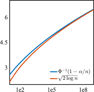
The following proposition gives an approximation of ${\Phi }^{-1}(-\alpha /n)$ for any $\alpha \in (0,1)$.

Max-Central Limit Theorem (Fisher–Tippett–Gnedenko) ^prop-max

Let $Z_i\stackrel{\text{iid}}{\sim }\mathcal{N}(0,1),i=1,\dots ,n$. We have

$$\frac{{\max }_i{Z}_i}{\sqrt{2\log n}}\stackrel{P}{\to }1,\text{as }n\to \infty .$$

Then, calculating the CDF of ${\max }_i{Z}_i$ gives

$$-{\Phi }^{-1}(\alpha /n)=\sqrt{2\log n}(1+o(1)),$$

where the Asymptotic Notation holds as $n\to \infty$.

^fig-a gives an illustration of how $\sqrt{2\log n}$ approximates ${\Phi }^{-1}(-\alpha /n)$ when $\alpha =0.05$.

Approximation of \Phi^{-1}(-\alpha/n).

Sparsity Connection

The previous proposition already connects the threshold of the Bonferroni algorithm to the max statistic, which is good for detecting sparse signals. The following propositions further formalize the connection between the Bonferroni algorithm and sparsity, suggesting that the Bonferroni algorithm is good at detecting sparse signals and dealing with sparse alternatives.

Proposition

If ${\theta }_1=(1+ϵ)\sqrt{2\log n}$ with $ϵ\in (0,1)$ and ${\theta }_i=0$ for $i\ge 2$, then the Bonferroni algorithm has power

$$\mathbb{P}(\underset{\text{reject }{H}_{0,1}}{\underbrace{1\in R=A(X)}})\to 1,\text{ as }n\to \infty .$$

Proof

First, by the definition of the Bonferroni algorithm, we have

$$\mathbb{P}(1\in R)=\mathbb{P}(X_1\ge -{\Phi }^{-1}(\alpha /n))=\mathbb{P}(Z\ge -{\Phi }^{-1}(\alpha /n)-{\theta }_1),$$

where $Z\sim \mathcal{N}(0,1)$. Then, by Proposition ^prop-max, we get

$$\mathbb{P}(Z\ge -{\Phi }^{-1}(\alpha /n)-{\theta }_1)=\mathbb{P}(Z\ge (1+o(1)-1-ϵ)\sqrt{2\log n}).$$

Letting $n\to \infty$ gives

$$\mathbb{P}(1\in \mathbb{R})\to \mathbb{P}(Z\ge -\infty )=1.$$

The following proposition can be obtained by a similar argument.

Proposition

If ${\theta }_1=(1-ϵ)\sqrt{2\log n}$ with $ϵ\in (0,1)$ and ${\theta }_i=0$ for $i\ge 2$, then the Bonferroni algorithm has power approaching 0 as $n\to \infty$.

Benjamini-Hochberg Algorithm

Let $p_{(1)}\le \cdots \le p_{(n)}$ be sorted p-values. The Benjamini-Hochberg (BH) algorithm returns

$$A(\vec{p})=\left\{(i):(i)\le \max \left\{i:p_{(i)}\le \frac{i}{n}\alpha \right\}\right\}.$$

That is, denoting $i_0:=\max \{i:p_{(i)}\le i\alpha /n\}$, we reject $i_0$ nulls with the smallest p-values.

Note that

$$A(\vec{p})\ne \left\{(i):p_{(i)}\le \frac{i}{n}\alpha \right\}.$$

That is, unlike Bonferroni, BH does not reject nulls under a function graph. Instead, it first determines $i_0$, and then reject nulls before $i_0$ on the line of sorted p-values. See ^fig-bh for an illustration: even before $i_0$ there are some p-values above the line $\frac{i}{n}\alpha$, they get rejected because $i_0$ is the last index below the line. Also note that without the bound’s dependence on $i$, the BH algorithm reduces to the Bonferroni algorithm.

Illustration of BH algorithm.

FDR control for BH

For independent p-values, the BH algorithm satisfies $\mathrm{FDR}\le \alpha \cdot \#\text{true nulls}/n\le \alpha$. The first equality holds when the p-values are uniformly distributed for true nulls.

Proof

We first define the confusion matrix:

#	Accepted	Rejected
True	$U$	$V$
False	$T$	$S$

And we denote $N$ as the index set of true nulls; $R$ is the rejection set as before. With a slight abuse of notation, we use $N$ and $R$ to also denote the number of true nulls and the number of rejections, respectively. Then, $U+V=N$, $T+S=n-N$, $U+T=n-R$, and $V+S=R$.

Define the indicator $V_i={\mathrm{𝟙}}_{\{i\in R\}}$. By definition, we have

$$\begin{array}{rl}\mathrm{FDR}=& \mathbb{E}\left[\frac{V}{1\vee R}\right]\\ =& \mathbb{E}\left[\sum _{i\in N}\frac{V_i}{1\vee R}\right]\\ =& \sum _{i\in N}\mathbb{E}\left[\sum _{k=1}^n\frac{V_i}{k}{\mathrm{𝟙}}_{\{R=k\}}\right].\end{array}$$

Without loss of generality, we assume the p-values are already sorted. Then, observe that if $i\in R$, there exists $j\ge i$ such that $p_i\le p_j\le \alpha j/n$. Therefore, if we consider a virtual instance where $p_i=0$ and other p-values are unchanged, BH will return the same rejection set for this instance.^[For this virtual instance, p-values may not be sorted anymore. However, p-values that are smaller than $p_j$ in the original instance will stay below $p_j$]. We denote $R(p_i\leftarrow 0)$ as the rejection set after setting $p_i$ to 0. Note that this virtual instance only depends on $p_{-i}=\{p_1,\dots ,p_{i-1},p_{i+1},\dots ,p_n\}$. Therefore,

$$\begin{array}{rl}\mathrm{FDR}=& \sum _{i\in N}\mathbb{E}\left[\sum _{k=1}^n\frac{1}{k}{V}_i{\mathrm{𝟙}}_{\{R(p_i\leftarrow 0)=k\}}\right]\\ =& \sum _{i\in N}\mathbb{E}\left[\sum _{k=1}^n\frac{1}{k}\mathbb{E}\left[V_i{\mathrm{𝟙}}_{\{R(p_i\leftarrow 0)=k\}}\mid p_{-i}\right]\right]\\ =& \sum _{i\in N}\mathbb{E}\left[\sum _{k=1}^n\frac{1}{k}\mathbb{P}\left(p_i\le \alpha \frac{k}{n}\right){\mathrm{𝟙}}_{\{R(p_i\leftarrow 0)=k\}}\right]\\ \le & \sum _{i\in N}\mathbb{E}\left[\sum _{k=1}^n\frac{1}{k}\cdot \alpha \frac{k}{n}\cdot {\mathrm{𝟙}}_{\{R(p_i\leftarrow 0)=k\}}\right]\\ =& \sum _{i\in N}\mathbb{E}\left[\frac{\alpha }{n}\right]\\ =& \frac{N}{n}\alpha \\ \le & \alpha ,\end{array}$$

where the first equation is because if $V_i=1$, setting $p_i=0$ will not change the rejection set as we argued; the second equation uses the tower property; the third equation uses the fact that $p_i$ is independent of $p_{-i}$, and the indicator specifies that $i_0=k$; the fourth inequality uses the fact that $p_i$ is super-uniform, and the equality holds when it’s uniform.

Connection Between Different Metrics

Using the confusion matrix, we can express the metrics as

$$\mathrm{FDR}=\mathbb{E}\left[\frac{V}{1\vee R}\right],\mathrm{FWER}=\mathbb{P}(V\ge 1)=\mathbb{E}[{\mathrm{𝟙}}_{\{V\ge 1\}}].$$

Since $R\ge V$, we have $1_{\{V\ge 1\}}\ge V/(1\vee R)$, and thus $\mathrm{FDR}\le \mathrm{FWER}$. For a single hypothesis test, or if we consider the global null, where we either reject all nulls or none, we have $V/(1\vee R)={\mathrm{𝟙}}_{\{V\ne \varnothing \}}={\mathrm{𝟙}}_{\{V\ge 1\}}$. In this case, $\mathrm{FDR}=\mathrm{FWER}$.